This post originally appeared on the ModelOp Tech Blog
If I could predict the future, some aspects of business would become much easier. For instance, if I owned a store and could somehow divine what my next week’s sales would look like, I could make sure that my inventory was perfectly matched to the coming demand. Similarly, if I could predict the movements of the stock market, I could use this information to make advantageous trades. Sadly, I can’t see into the future. So the natural question becomes: what are the best predictions I can make about the future given the information that is available to me today?
This is where the statistical field of forecasting comes in. In its most basic form, the goal is this: given a time-indexed list of numbers (for instance, a stock ticker or the weekly sale numbers of a product), what are the best estimates I can make of future values of the series (e.g. the stock’s next price or tomorrow’s sales)? Note that for the purposes of this blog post, we will be dealing only with the time series itself - no other data will be used. One might hope that if I knew, say, the rate of inflation I might be better able to predict shifts in the stock market. But that is a topic for another post.
Since it’s getting cold in Chicago and I’m dreaming of warmer days, lets take our time series to be the historical high temperature at Chicago’s O’Hare Airport. We’ll try to build a model that can predict the average high temperature next month from this historical data.
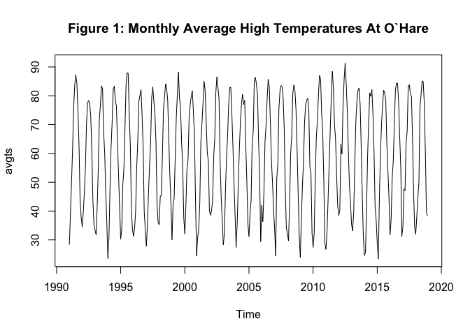
We get our data from the National Centers for Environmental information. It consists of the daily high temperatures at O’Hare airport from 1991 to the present, averaged by month. We then create an R ts() object containing just this information. It is plotted in Figure 1 below.
Before we even begin trying to model anything, let’s make a few observations. First, we can see that all of these numbers lie between (say) 20 and 95 degrees Fahrenheit. So an ideal model for this data would have outputs roughly in these ranges. If our model is regularly predicting 110 or -15 degrees for the monthly average high temperature, we would already be able to say that it’s not a very good model. This may seem obvious, but it should be thought of as a toy example of how past data can tell us something about how we should forecast.
Second, we can see that there is a cyclical nature to the data - highs are lower in the winters and higher in the summers. This is a phenomenon known (for obvious reasons) as seasonality in time-series modeling. An ideal model would take this into account. The effect of seasonality is extremely pronounced here (compare to, say, a stock price where the effect of the time of year presumably does not show up nearly as strongly). Finally, there doesn’t seem to be any particularly strong trend in these numbers - the ranges remain roughly constant throughout the time period we’re looking at.
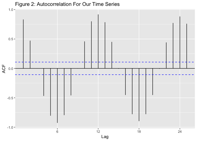
One thing that we can look at with time series data is something called the autocorrelation - roughly, how much are the values of the time series correlated with the surrounding values. The plot of our autocorrelation function is included below as Figure 2. As we can see, the value for a month is highly correlated with the same month in different years, slightly less correlated with the surrounding months, and has negative correlation roughly 6 months ahead. This tells us that this series is strongly seasonal.
Alright, we’ve explored the data a bit - let’s try to build a model. First, we want to get some baselines for our predictions. These are usually naive prediction methods that we will compare our future, fancier models against - if we can’t beat the baselines with our fancy model, then the fancy model probably isn’t worth much.
First, what’s the most naive prediciton method we could use? Well, we could just always predict the last value we saw. In fact, this is known as the naive method. The issue with this is that it will consistently over/under estimate in this case - basically, we’re not using the seasonality of the data in any way. Another option that doesn’t really use the seasonality in any way is to take the mean over some prior period (say, 3 months) and use that as the prediction. We might expect that this does slightly better than the naive method, but again we’re not really incorporating the seasonality. The final baseline we’ll look at is the seasonal naive method - namely, predict the value of the series from 12 months ago as the prediction. We might expect that this does pretty well with this time series.
Let’s see how each of these does for 2018.
actual <- window(avgts,2018)
naive <- window((stats::lag(avgts,-1)),2018,c(2018,12))
mean <- window(rollapply(avgts, 3, "mean", align = "right", partial = T, fill = NA),2018)
seasonal <- window(stats::lag(avgts,-12),2018,c(2018,12))
actual

##           Jan      Feb      Mar      Apr      May      Jun      Jul
## 2018 31.87097 38.00000 44.70968 50.03333 76.35484 80.43333 85.12903
##           Aug      Sep      Oct      Nov      Dec
## 2018 84.80645 77.50000 60.67742 39.73333 38.25000

mean

##           Jan      Feb      Mar      Apr      May      Jun      Jul
## 2018 37.66595 34.68817 38.19355 44.24767 57.03262 68.94050 80.63907
##           Aug      Sep      Oct      Nov      Dec
## 2018 83.45627 82.47849 74.32796 59.30358 46.22025

naive

##           Jan      Feb      Mar      Apr      May      Jun      Jul
## 2018 34.19355 31.87097 38.00000 44.70968 50.03333 76.35484 80.43333
##           Aug      Sep      Oct      Nov      Dec
## 2018 85.12903 84.80645 77.50000 60.67742 39.73333

seasonal

##           Jan      Feb      Mar      Apr      May      Jun      Jul
## 2018 34.58065 47.67857 47.12903 63.76667 67.70968 83.26667 83.80645
##           Aug      Sep      Oct      Nov      Dec
## 2018 80.74194 79.73333 65.45161 46.93333 34.19355
For our evaluation metric, lets look at mean absolute error (MAE) - the average of the absoulte values of the errors of the predictions.
naiveMAE <- mean(abs(actual-naive))
meanMAE <- mean(abs(actual-mean))
seasonalMAE <- mean(abs(actual-seasonal))
naiveMAE

## [1] 8.538306

meanMAE

## [1] 8.686111

seasonalMAE

## [1] 5.305876
As expected, the seasonal naive method outperforms the other two. However, lets see if we can do better.
Everything we’ve done so far is fairly straightforward. A much fancier method of time series forecasting is the ARIMA method. Such a model consists of several parts - first the autoregressive (AR) piece takes weighted sums of some number of previous observations (we can think of this as a much more general version of the naive method we looked at above). The next piece is the integrated (I) piece, which takes difference of the series to force it to have nicer statistical properties. Finally, there’s the moving average (MA) piece, which takes weighted sums of white-noise errors of previous terms. If we combine these all together (plus seasonal analogues of these), we get a general ARIMA model.
This might seem like a lot to deal with, but luckily the forecast package in R has a function that computes such a model for you.
train <- window(avgts, end=c(2017,12))
trainmodel <- auto.arima(train)
trainmodel

## Series: train
## ARIMA(2,0,2)(1,1,0)[12] with drift
##
## Coefficients:
##           ar1     ar2     ma1      ma2     sar1   drift
##       -0.0746  0.7579  0.3338  -0.6444  -0.4218  0.0024
## s.e.   0.0828  0.0689  0.0992   0.0944   0.0524  0.0345
##
## sigma^2 estimated as 23.15:  log likelihood=-931.66
## AIC=1877.31   AICc=1877.68   BIC=1903.51
Let’s break down what this means: the (2,0,2) means the fit model has 2 AR terms, 0 differences (the I part of the model), and 2 MA terms. The (1,1,0) piece corresponds to the seasonal ARIMA terms - one AR term, and one difference. The [12] indicates the seasonality - since there are 12 months in a year, this is the natural choice. Finally, the model incorporates slight drift - a trend in the data. The coefficients and standard errors for each pieces are then listed, as well as some statistics about the fit of the model.
Let’s see how this model does at predicting for 2018:
fullmodel <- Arima(avgts,model=trainmodel)
arimaforecast <- tail(fullmodel$fitted,12)
arimaforecast

##           Jan      Feb      Mar      Apr      May      Jun      Jul
## 2018 33.43440 41.00933 48.22833 58.20269 65.85530 82.51868 82.58382
##           Aug      Sep      Oct      Nov      Dec
## 2018 82.65571 78.56760 65.93328 48.73150 30.35375

arimaMAE <- mean(abs(actual-arimaforecast))
arimaMAE

## [1] 4.729957
So this model outperforms the seasonal naive method, but not by much. There’s definitely a tradeoff between the simplicity of the model and making marginal gains that is problem dependent.
That does it for this brief intro to forecasting. It is a topic that certainly will come up again in future blog posts. If you want to learn more about what was covered here (plus a plethora of other topics in this space), a good reference is Forecasting: Principles and Practices by Rob J Hyndman and George Athanasopoulos, which is available freely online.